Module 6
Scan: Outliers
Overview
Summary
In statistics, an outlier is defined as an observation which stands far away from the most of other observations. An outlier can be a result of a measurement error and the inclusion of that error would have a great impact on the analysis results. Therefore, every data set should be scanned for possible outliers before conducting any statistical analysis. Like missing values, detecting outliers and dealing with them are also crucial in the data preprocessing. In this module, first you will learn how to identify univariate and multivariate outliers using descriptive, graphical and distance-based methods. Then, you will learn different approaches to deal with these values using R.
Learning Objectives

The learning objectives of this module are as follows:
- Identify the outlier(s) in the data set.
- Apply descriptive methods to identify univariate outliers.
- Apply graphical approaches to scan for univariate or multivariate outliers.
- Apply distance-based metrics to identify univariate or multivariate outliers.
- Learn commonly used approaches to handle outliers.
Outliers
In statistics, an outlier is defined as an observation which stands
far away from most of the other observations. An outlier deviates so
much from other observations as to arouse suspicion that is was
generated by a different mechanism (Hawkins
(1980)). Let’s take an example. Assume that we are interested in
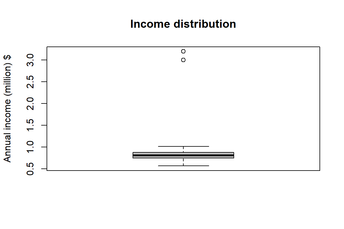
customer profiling and we find out that the average annual income of our
customers is 800K. But there are two customers having annual income of 3
and 3.2 million dollars. These two customers’ annual income is much
higher than rest of the customers (see the boxplot below). These two
observations will be seen as outliers.
Types of Outliers
Outlier can be univariate and multivariate. Univariate
outliers can be found when looking at a distribution of values
in a single variable. The example given above is an example of a
univariate outlier as we only look at the distribution of income (i.e.,
one variable) among our customers. On the other hand,
multivariate outliers can be found in a n-dimensional
space (of n-variables). In order to find them, we need to look at
distributions in multi-dimensions.
To illustrate multivariate outliers, let’s assume that we are
interested in understanding the relationship between height and weight.
Below, we have univariate and bivariate distribution for Height and
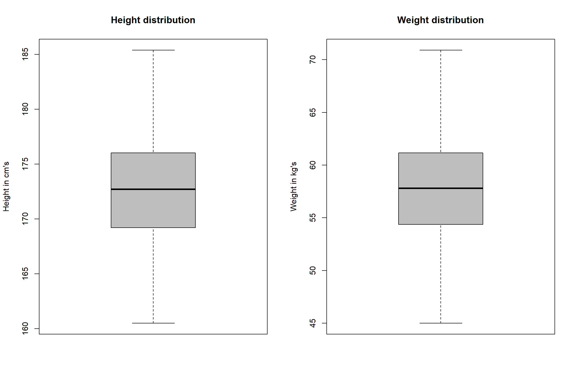
Weight. When we look at the univariate distributions of Height and
Weight (i.e., using boxplots) separately, we don’t spot any abnormal
cases (i.e. above and below the \(1.5\times
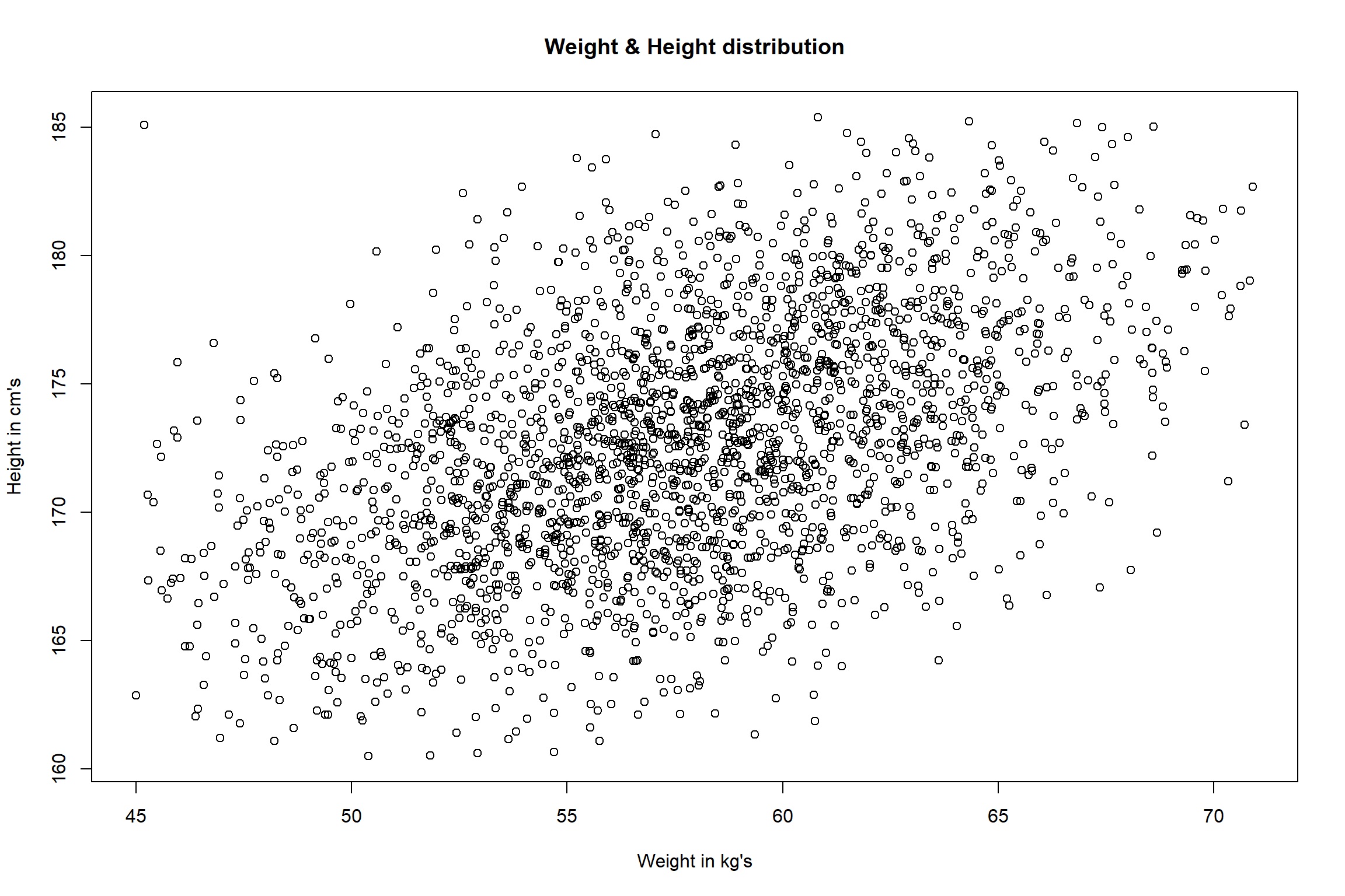
IQR\) fence). However, when we look at the bivariate (two
dimensional) distribution of Height and Weight (using scatter plot), we
can see that we have one observation whose weight is 45.19 kg and height
is 185.09 (on the upper-left side of the scatter plot). This observation
is far away from most of the other weight and height combinations thus,
will be seen as a multivariate outlier.
Most Common Causes of Outliers
Often an outlier can be a result of data entry errors, measurement errors, experimental errors, intentional errors, data processing errors or due to the sampling (i.e., sampling error). The following are the most common causes of outliers (taken from: https://www.analyticsvidhya.com/blog/2016/01/guide-data-exploration/)
Data Entry Error: Outliers can arise because of the human errors during data collection, recording, or entry.
Measurement Error: It is the most common source of outliers. This is caused when the measurement instrument used turns out to be faulty.
Experimental Error: Another cause of outliers is the experimental error. Experimental errors can arise during data extraction, experiment/survey planning and executing errors.
Intentional Error: This type of outlier is commonly found in self-reported measures that involves sensitive data. For example, teens would typically under report the amount of alcohol that they consume. Only a fraction of them would report actual value. Here actual values might look like outliers because rest of the teens are under reporting the consumption.
Data Processing Error: Often, due to the data sets are extracted from multiple sources, it is possible that some manipulation or extraction errors may lead to outliers in the data set.
Sampling Error: Sometimes, outliers can arise due to the sampling (taking samples from population) process. Typically, this type of outliers can be seen when we take a few observations as a sample.
Detecting Outliers
Outliers can drastically change the results of the data analysis and statistical modelling. Some of the unfavourable impacts of outliers are as follows:
- They increase the error variance.
- They reduce the power of statistical tests.
- They can bias or influence the estimates of model parameters that
may be of substantive interest.
Therefore, one of the most important tasks in data preprocessing is
to identify and properly handle the outliers.
There are many methods developed for outlier detection. Majority of them deal with numerical data. This module will introduce the most basic ones with their application using R packages.
Univariate Outlier Detection Methods
One of the simplest methods for detecting univariate outliers is the
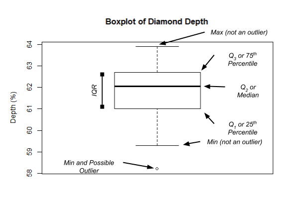
use of boxplots. A boxplot is a graphical display for describing the
distribution of the data using the median, the first (Q1) and third
quartiles (Q3), and the inter-quartile range (\(IQR = Q3 - Q1\)). Below is an illustration
of a typical boxplot (taken from [Dr. James Baglin’s Intro to Stats
website] (https://astral-theory-157510.appspot.com/secured/MATH1324_Module_02.html#box_plots)).
In the boxplot, the “Tukey’s method of outlier
detection” is used to detect outliers. According to this
method, outliers are defined as the values in the data set that fall
beyond the range of \(-1.5 \times IQR\)
to \(1.5 \times IQR\). These \(-1.5 \times IQR\) and \(1.5 \times IQR\) limits are called “outlier
fences” and any values lying outside the outlier fences are depicted
using an “o” or a similar symbol on the boxplot.
Note that Tukey’s method is a nonparametric way of detecting
outliers, therefore it is mainly used to test outliers in non-symmetric/
non-normal data distributions.
In order to illustrate the boxplot, we will use the Diamonds.csv data set available under the
data repository.
Diamonds <- read.csv("data/Diamonds.csv")
head(Diamonds)
## carat cut color clarity depth table price x y z
## 1 0.23 Ideal E SI2 61.5 55 326 3.95 3.98 2.43
## 2 0.21 Premium E SI1 59.8 61 326 3.89 3.84 2.31
## 3 0.23 Good E VS1 56.9 65 327 4.05 4.07 2.31
## 4 0.29 Premium I VS2 62.4 58 334 4.20 4.23 2.63
## 5 0.31 Good J SI2 63.3 58 335 4.34 4.35 2.75
## 6 0.24 Very Good J VVS2 62.8 57 336 3.94 3.96 2.48We can use boxplot() function (under Base graphics) to
get the boxplot of the carat variable:
Diamonds$carat %>% boxplot(main="Boxplot of Diamond Carat", ylab="Carat", col = "grey")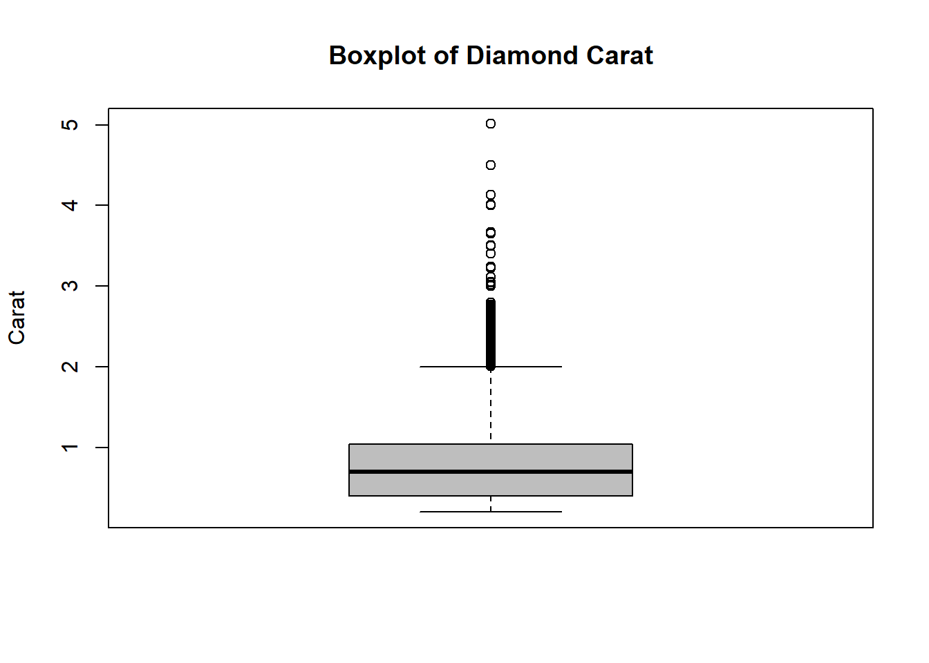
According to the Tukey’s method, the carat variable
seems to have many outliers. In the next section, we will discuss
different approaches to handle these outliers.
There are also distance based methods to detect univariate outliers.
One of them is to use the \(z\)- scores
(i.e., normal scores) method. In this method, a standardised score
(\(z\)-score) of all observations are
calculated using the following equation:
\[ z_i = \frac{X_i - \bar{X}}{S}\]
In the equation below, \(X_i\)
denotes the values of observations, \(\bar{X}\) and \(S\) are the sample mean and standard
deviation, respectively. An observation is regarded as an outlier based
on its \(z\)-score, if the absolute
value of its \(z\)-score is
greater than 3.
Note that, z-score method is a parametric way of detecting outliers and assumes that the underlying data is normally distributed. Therefore, if the distribution is not approximately normal, this method shouldn’t be used.
In order to illustrate the \(z\)-
score approach, we will use the “outliers package”. The
outliers package provides several useful functions to systematically
extract outliers. Among those, the scores() function will
calculate the \(z\)-scores (in addition
to the \(t\), chi-square, IQR, and
Median absolute deviation scores) for the given data. Note that, there
are many alternative functions in R for calculating \(z\)-scores. You may also use these
functions and detect the outliers.
Let’s investigate any outliers in the depth variable
using \(z\)-score approach. First, we
will make sure that the depth distribution is approximately
normal. For this purpose we can use histogram (or
boxplot()) to check the distribution:
hist(Diamonds$depth)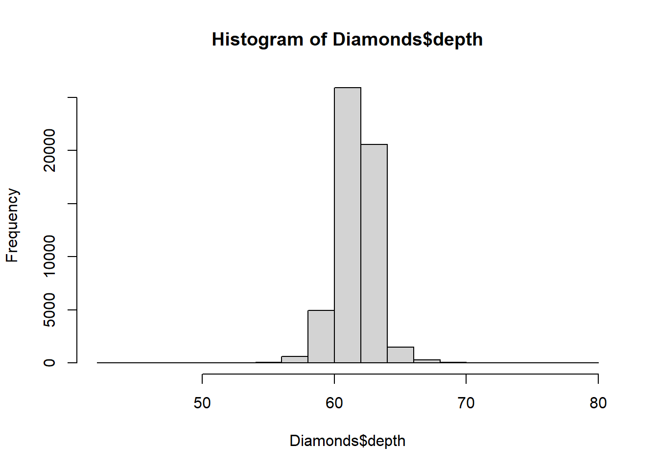
After confirming the depth variable has an approximately
normal distribution, we can calculate z scores using outliers
package:
library(outliers)
z.scores <- Diamonds$depth %>%  scores(type = "z")
z.scores %>% summary()
## Min. 1st Qu. Median Mean 3rd Qu. Max.
## -13.08748 -0.52310 0.03532 0.00000 0.52393 12.04128From the summary() output, we can see that the minimum z
score is -13.08 and the maximum is 12.04.
Using which(), we can also find the locations of the
\(z\)-scores whose absolute value is
greater than 3.
# Finds the locations of outliers in the depth variable

which(abs(z.scores) >3 )
## [1] 3 92 98 205 222 228 299 353 370 386 424 441
## [13] 444 529 636 713 714 715 720 751 772 778 802 840
## [25] 896 899 900 920 930 939 940 1099 1228 1239 1268 1439
## [37] 1600 1609 1676 1683 1796 1811 1812 1883 1907 2016 2025 2026
## [49] 2086 2113 2132 2178 2183 2184 2213 2217 2230 2314 2337 2353
## [61] 2357 2367 2412 2447 2480 2498 2505 2582 2584 2699 2746 2874
## [73] 2890 2914 2935 2982 2991 3152 3185 3421 3447 3565 3597 3754
## [85] 3837 4024 4145 4152 4208 4274 4308 4326 4327 4328 4416 4506
## [97] 4513 4519 4602 4655 4669 4696 4780 4789 4808 4886 4925 4971
## [109] 4972 5005 5007 5015 5034 5140 5354 5447 5461 5463 5470 5499
## [121] 5558 5576 5591 5699 5707 5740 5744 5776 5846 5870 5922 5935
## [133] 6021 6061 6163 6166 6341 6342 6348 6402 6430 6466 6493 6503
## [145] 6564 6628 6631 6656 6678 6741 6752 6796 6813 6816 6920 6940
## [157] 6971 6994 7023 7024 7097 7102 7172 7375 7417 7594 7675 7700
## [169] 7705 7738 7774 7821 7901 8010 8015 8160 8187 8188 8203 8357
## [181] 8393 8412 8456 8509 8576 8620 8673 8722 8854 8856 8866 8890
## [193] 8894 9098 9121 9282 9465 9604 9677 9735 9785 9874 9908 9950
## [205] 9981 9982 9983 10172 10271 10291 10378 10465 10474 10498 10594 10657
## [217] 10658 10690 10761 10814 10937 10962 11091 11114 11130 11161 11242 11313
## [229] 11370 11628 11758 11779 11828 11911 12132 12187 12233 12270 12281 12424
## [241] 12477 12619 12646 12815 12830 13003 13126 13222 13248 13270 13271 13279
## [253] 13563 13724 13758 13923 13992 13993 14039 14114 14129 14139 14456 14505
## [265] 14646 14668 14848 14882 14914 15000 15062 15147 15228 15314 15350 15504
## [277] 15624 15644 15670 15685 15782 15812 15816 15850 15866 15941 16085 16123
## [289] 16257 16328 16409 16440 16502 16505 16534 16638 16858 17025 17098 17182
## [301] 17197 17223 17314 17476 17482 17490 17553 17594 17692 17718 17720 17957
## [313] 18025 18073 18358 18359 18462 18531 18545 18686 18816 19016 19153 19184
## [325] 19247 19289 19332 19347 19407 19503 19590 19786 19793 19985 20103 20338
## [337] 20442 20648 20878 21157 21449 21513 21574 21602 21603 21685 21712 21713
## [349] 21737 22005 22030 22052 22461 22573 22594 22621 22668 22732 22742 22756
## [361] 22832 22872 23021 23176 23196 23287 23289 23490 23568 23645 24036 24242
## [373] 24245 24349 24524 24599 24892 24992 25025 25138 25281 25341 25351 25389
## [385] 25441 25452 25566 25730 25900 26067 26100 26249 26264 26265 26389 26432
## [397] 26491 26560 26651 27165 27352 27624 27634 27647 28271 30045 30375 30719
## [409] 30720 31231 31245 31251 31616 32073 32470 32507 32902 33016 33017 33103
## [421] 33524 33920 34252 34582 34699 35073 35119 35233 35663 35915 36044 36504
## [433] 36571 36673 36818 36819 36822 36835 36933 36959 37112 37217 37220 37276
## [445] 37304 37330 37506 37677 37678 37699 37701 37746 37781 37814 38041 38042
## [457] 38054 38154 38174 38315 38443 38550 38642 38841 39061 39088 39220 39254
## [469] 39308 39319 39386 39566 39679 39739 39842 39907 39914 40019 40026 40330
## [481] 40419 40421 40422 40434 40474 40485 40531 40615 40674 40695 40709 40767
## [493] 40772 40875 40900 40970 41061 41126 41331 41504 41506 41547 41660 41695
## [505] 41776 41821 41842 41857 41878 41919 42013 42092 42105 42120 42142 42192
## [517] 42257 42394 42447 42513 42548 42575 42644 42718 42805 42903 42905 42987
## [529] 42988 43177 43217 43386 43399 43481 43584 43706 43716 43777 43847 44040
## [541] 44155 44158 44212 44501 44533 44867 45035 45058 45067 45251 45535 45615
## [553] 45689 45760 45829 46093 46203 46346 46348 46361 46379 46431 46450 46477
## [565] 46558 46574 46611 46666 46680 46716 46785 46791 46824 46843 46891 46911
## [577] 47110 47126 47304 47604 47741 47776 47783 47912 47920 48093 48132 48242
## [589] 48260 48489 48499 48558 48607 48627 48706 48745 48855 48885 49100 49208
## [601] 49250 49265 49496 49508 49539 49653 49719 49774 49806 49883 49940 50004
## [613] 50039 50328 50380 50522 50583 50603 50747 50774 50907 51008 51049 51086
## [625] 51118 51123 51125 51140 51151 51203 51259 51392 51425 51463 51465 51497
## [637] 51514 51572 51622 51629 51692 51709 51718 51732 51840 51869 51929 51971
## [649] 52040 52084 52112 52245 52269 52345 52394 52460 52471 52475 52539 52566
## [661] 52569 52590 52594 52676 52677 52704 52707 52806 52849 52861 52862 52994
## [673] 53065 53123 53155 53435 53496 53541 53543 53661 53728 53757 53758 53801
## [685] 53864# Finds the total number of outliers according to the z-score
length (which(abs(z.scores) >3 ))## [1] 685According to the \(z\)-score method,
the depth variable has 685 outliers.
There are also many statistical tests to detect outliers. Some of
them are the Chi-square test for outliers, the Cochran’s test, the Dixon
test and the Grubbs test. In this course, we won’t cover these
statistical testing approaches used for detecting outliers. You may
refer to the [outliers package manual] (https://cran.r-project.org/web/packages/outliers/outliers.pdf)
which includes useful functions for the commonly used outlier tests as
well as the distance-based approaches.
Multivariate Outlier Detection Methods
When we have only two variables, the bivariate visualisation
techniques like bivariate boxplots and scatter plots, can easily be used
to detect any outliers.
To illustrate the bivariate, we will assume that we are only
interested in one numerical carat variable and a one factor
(quantitative) cut variable in the Diamonds data set.
boxplot(Diamonds$carat ~ Diamonds$cut, main="Diamond carat by cut", ylab = "Carat", xlab = "Cut")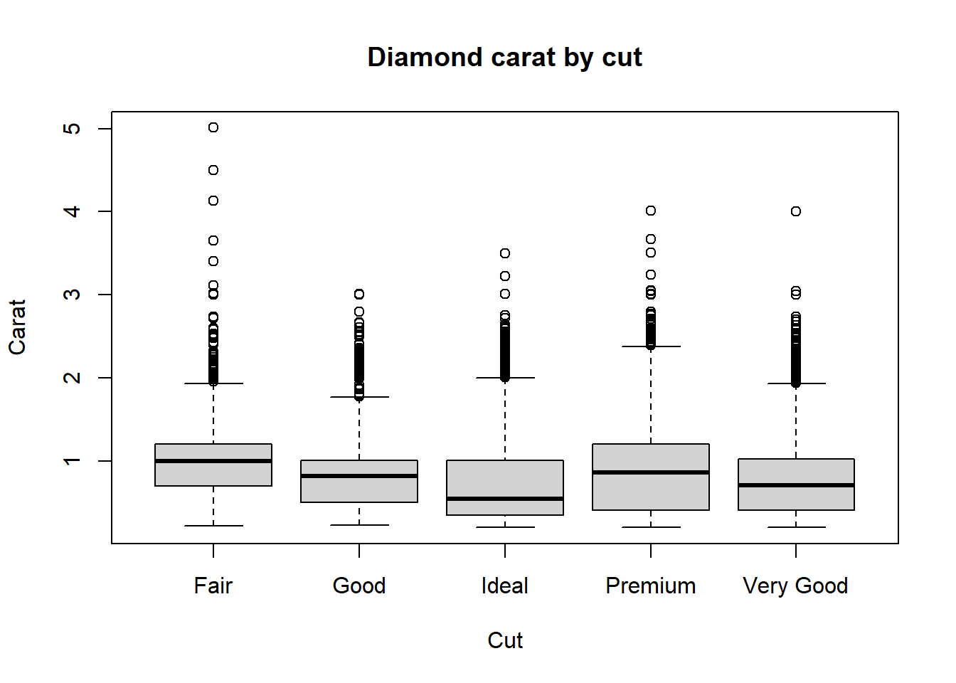
Using the univariate boxplot approach, we can easily detect outliers
in carat for a given cut.
Another bivariate visualisation method is the scatter plots. These
plots are used to visualise the relationship between two quantitative
variables. They are also very useful tools to detect obvious outliers
for the two-dimensional data (i.e., for two continuous variables).
The plot() function will be used to get the scatter plot
and detect outliers in carat and depth
variables:
Diamonds %>% plot(carat ~ depth, data = ., ylab="Carat", xlab="Depth", main="Carat by Depth")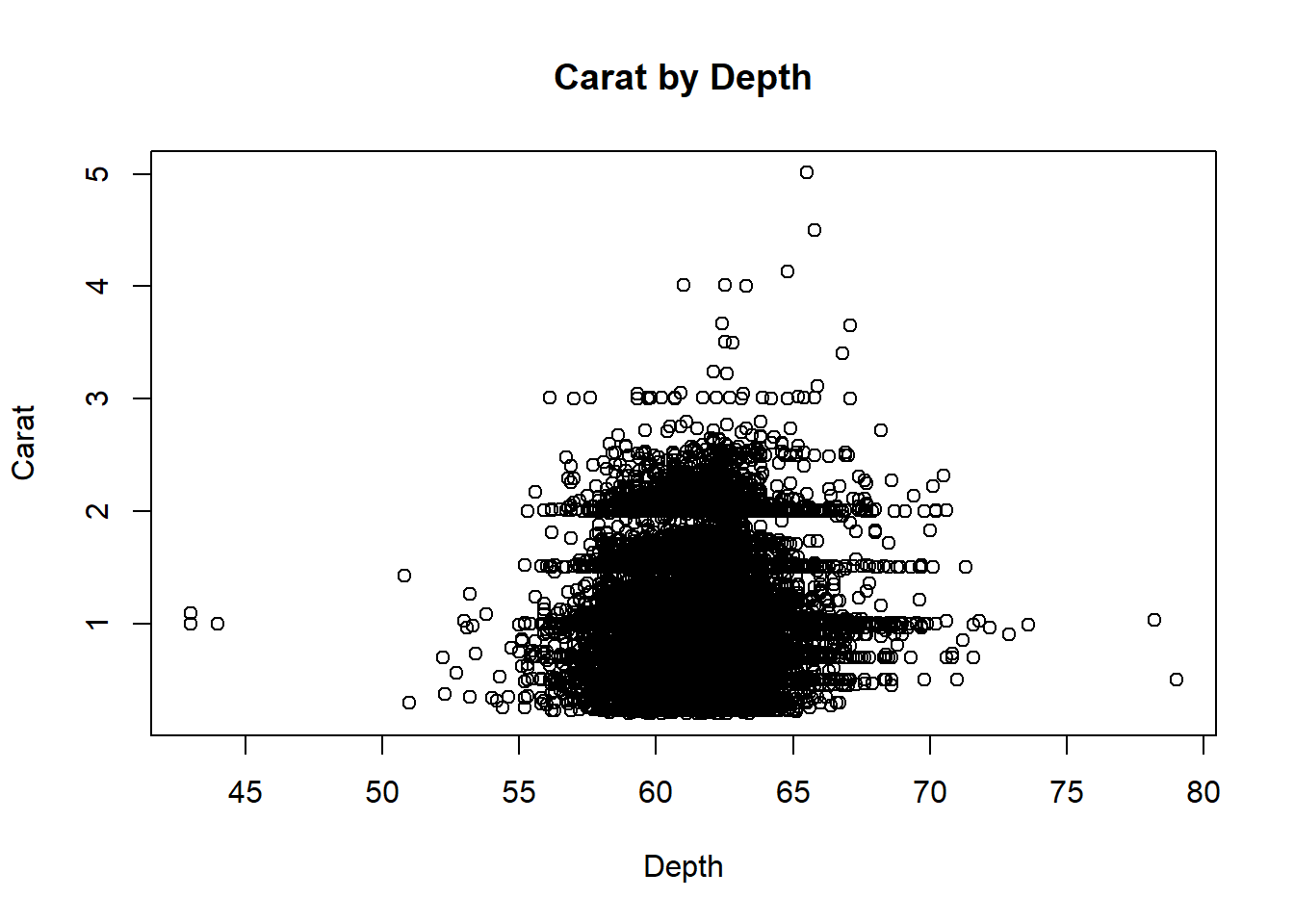
According to the scatter plot, there are some possible outliers on
the lower left (the data points where both carat and depth is small) and
lower right-hand side of the scatter (the data points with larger depth
but small carat values).
Scatter plots are useful methods to detect abnormal observations for
a given pair of variables. However, when there are more than two
variables, scatter plots can no longer be used. For such cases,
multivariate distance-based methods of outlier detection can be
used.
The Mahalanobis distance is the most commonly used
distance metric to detect outliers for the multivariate setting. The
Mahalanobis distance is simply an extension of the univariate \(z\)-score, which also accounts for the
correlation structure between all the variables. Mahalanobis distance
follows a Chi-square distribution with n (number of variables) degrees
of freedom, therefore any Mahalanobis distance greater than the
critical chi-square value is treated as outliers.
I will not go into details of calculation of the Mahalanobis
distance. We will use the MVN package to get these
distances as it will also provide us the useful Mahalanobis distance
vs. Chi-square quantile distribution plot (QQ plot) and contour plots.
For more information on this package and its capabilities please refer
to the paper on https://cran.r-project.org/web/packages/MVN/MVN.pdf.
To illustrate the usage of this package to detect multivariate
outliers, we will use a subset of the Iris
data, which is versicolor flowers, with the first three variables
(Sepal.Length, Sepal.Width and
Petal.Length).
First let’s read the data using:
# load iris data and subset using versicolor flowers, with the first three variables

iris <- read.csv("data/iris.csv")
versicolor <- iris %>%  filter(Species == "versicolor" ) %>%  dplyr::select(Sepal.Length, Sepal.Width, Petal.Length)
head(versicolor)
## Sepal.Length Sepal.Width Petal.Length
## 1 7.0 3.2 4.7
## 2 6.4 3.2 4.5
## 3 6.9 3.1 4.9
## 4 5.5 2.3 4.0
## 5 6.5 2.8 4.6
## 6 5.7 2.8 4.5The mvn() function under MVN package (Korkmaz, Goksuluk, and Zararsiz (2014)) lets us
to define the multivariate outlier detection method using the
multivariateOutlierMethod argument. When we use
multivariateOutlierMethod = "quan" argument, it detects the
multivariate outliers using the chi-square distribution critical value
approach mentioned above. The showOutliers = TRUE argument
will depict any multivariate outliers and show them on the QQ
plot.
# Multivariate outlier detection using Mahalanobis distance with QQ plots

results <- mvn(data = versicolor, multivariateOutlierMethod = "quan", showOutliers = TRUE)
As we can see on the QQ plot, the Mahalonobis distance suggests
existence of four outliers for this subset of the iris data.
If we would like to see the list of possible multivariate outliers,
we can use result$multivariateOutliers to select only the
results related to outliers as follows:
results$multivariateOutliers## Observation Mahalanobis Distance Outlier
## 34 34 14.065 TRUE
## 19 19 13.360 TRUE
## 23 23 12.005 TRUE
## 49 49 11.729 TRUEThis output is very useful in terms of providing the locations of
outliers in the data set. In our example the 34st, 19th, 23rd and 49th
observations are the suggested outliers for this subset of iris
data.
The mvn() function has also different plot options to
help discovering possible multivariate outliers. For example, to get the
bivariate contour plots, we can use
multivariatePlot = "contour" argument. However, note that
contour plots can only be used for two variables.
Let’s illustrate the contour plots on the subset of setosa flowers,
with the first two variables, Sepal.Length and
Sepal.Width.
# load iris data and subset using setosa flowers, with the first two variables

setosa <- iris %>%  filter( Species == "setosa" ) %>%  dplyr::select(Sepal.Length, Sepal.Width)
head(setosa)
## Sepal.Length Sepal.Width
## 1 5.1 3.5
## 2 4.9 3.0
## 3 4.7 3.2
## 4 4.6 3.1
## 5 5.0 3.6
## 6 5.4 3.9# Multivariate outlier detection using Mahalanobis distance with contour plots
results <- mvn(data = setosa, multivariateOutlierMethod = "quan", multivariatePlot = "contour")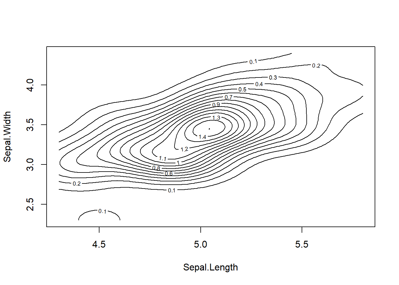
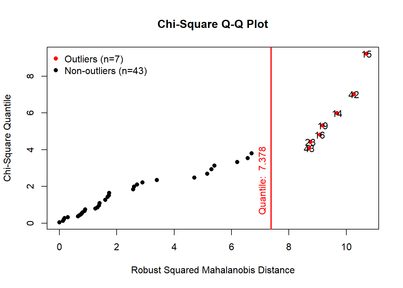
From the contour plot, we can see one anomality on the left-hand side
of the plot, however, according to the QQ plot, this abnormal case
doesn’t seem to be an outlier as its Mahanolobis distance didn’t exceed
the threshold chi-square value.
The Minimum Covariance Determinant (MCD) is another
approach for multivariate outliers. The cov.mcd function
under MASS package lets us to define the multivariate outlier detection
method. For more information on this function please refer to the paper
Detecting
multivariate outliers written by Leys, C. et.al. (2018) and the
samples from Handling
Multivariate Outliers.
Some applications of univariate and multivariate outlier detection
can extend from fraud detection (i.e., unusual purchasing behaviour of a
credit card owner), medicine (i.e. detection of unusual symptoms of a
patient), sports statistics (i.e., abnormal performance for players may
indicate doping), measurement errors (i.e., abnormal values could
provide an indication of a measurement error), etc. Like missing value
analysis, univariate and multivariate outlier analyses are also broader
concepts. There are also different distance-based and probabilistic
methods (like clustering analysis, genetic algorithm, etc.) that can be
used to detect outliers in the high dimensional data sets. There is a
huge theory behind the outlier detection methods and outlier analysis
would be a standalone topic of another course. Interested readers may
refer to the “Outlier analysis, by Charu C. Aggarwal” for the theory
behind the outlier detection methods (Aggarwal
(2015)).
Approaches to Handling Outliers
Most of the ways to deal with outliers are similar to the methods of
missing values like deleting them or imputing some values (i.e., mean,
median, mode) instead. There are also other approaches specific to
dealing with outliers like capping, transforming, and binning them.
Here, we will discuss the common techniques used to deal with outliers.
Some of the methods mentioned in this Module (like transforming and
binning) will be covered in the next module (Module 7: Transform),
therefore I won’t go into the details of transforming and binning
here.
Excluding or Deleting Outliers
Some authors recommend that if the outlier is due to data entry
error, data processing error or outlier observations are very small in
numbers, then leaving out or deleting the outliers would be used as a
strategy. When this is the case, we can exclude/delete outliers in a
couple different ways.
To illustrate, let’s revisit the outliers in the carat
variable. Remember that we already found the locations of the outliers
in the carat variable using which() function.
Intuitively, we can exclude these observations from the data
using:
Carat_clean<- Diamonds$carat[ - which( abs(z.scores) >3 )]Let’s see another example on the previous versicolor
data:
versicolor <- iris %>%  filter(Species == "versicolor" ) %>%  dplyr::select(Sepal.Length, Sepal.Width,Petal.Length)
head(versicolor)
## Sepal.Length Sepal.Width Petal.Length
## 1 7.0 3.2 4.7
## 2 6.4 3.2 4.5
## 3 6.9 3.1 4.9
## 4 5.5 2.3 4.0
## 5 6.5 2.8 4.6
## 6 5.7 2.8 4.5results <- mvn(data = versicolor, multivariateOutlierMethod = "quan", showOutliers = TRUE)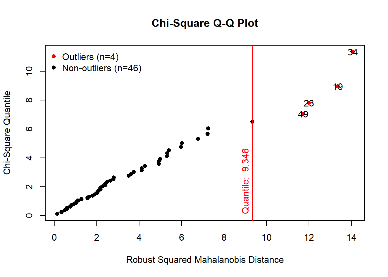
results$multivariateOutliers## Observation Mahalanobis Distance Outlier
## 34 34 14.065 TRUE
## 19 19 13.360 TRUE
## 23 23 12.005 TRUE
## 49 49 11.729 TRUEThe Mahalonobis distance method provided us the locations of outliers
in the data set. In our example the 34st, 19th, 23rd and 49th
observations are the suggested outliers. Using the basic filtering and
subsetting functions, we can easily exclude these two outliers:
# Exclude 34st, 19th, 23rd and 49th observations

versicolor_clean <- versicolor[ -c(19,23,34,49), ]

# Check the dimension and see outliers are excluded

dim(versicolor_clean)
## [1] 46 3Note that, the mvn() function also has an argument
called showNewData = TRUE to exclude the outliers. One can
simply detect and remove outliers using the following argument:
versicolor_clean2 <- mvn(data = versicolor, multivariateOutlierMethod = "quan", showOutliers = TRUE, showNewData = TRUE)
# Prints the data without outliers

dim(versicolor_clean2$newData)
## [1] 46 3Imputing
Like imputation of missing values, we can also impute outliers. We
can use mean (need to be used with caution!), median imputation or
capping methods to replace outliers. Before imputing values, we should
analyse the distribution carefully, and investigate whether the
suggested outlier is a result of data entry/processing error. If the
outlier is due to a data entry/processing error, we can go with imputing
values.
For the illustration purposes, let’s replace the two outlier values
in carat variable with its mean by using Base R
functions:
Diamonds <- read.csv("data/Diamonds.csv")
Diamonds$carat[ which( abs(z.scores) >3 )] <- mean(Diamonds$carat, na.rm = TRUE)
Replacing outliers with the median or a user specified value can also be done using a similar approach. Note that, you may also prefer to write your own functions to deal with outliers.
Capping (a.k.a Winsorising)
Capping or winsorising involves replacing the outliers with the nearest neighbours that are not outliers. For example, for outliers that lie outside the outlier fences on a boxplot, we can cap it by replacing those observations outside the lower limit with the value of 5th percentile and those that lie above the upper limit, with the value of 95th percentile.
In order to cap the outliers we can use a user-defined function as follows (taken from: Stackoverflow):
# Define a function to cap the values outside the limits

cap <- function(x){
    quantiles <- quantile( x, c(.05, 0.25, 0.75, .95 ) )
    x[ x < quantiles[2] - 1.5*IQR(x) ] <- quantiles[1]
    x[ x > quantiles[3] + 1.5*IQR(x) ] <- quantiles[4]
    x}
To illustrate capping we will use the Diamond data set. In order to
cap the outliers in the carat variable, we can simply apply
our user-defined function to the carat variable as
follows:
Diamonds <- read.csv("data/Diamonds.csv")
carat_capped <- Diamonds$carat %>% cap()
We can also apply this function to a data frame using
sapply function. Here is an example of applying
cap() function to a subset of the Diamonds data frame:
# Take a subset of Diamonds data using quantitative variables

Diamonds_sub <- Diamonds %>%  dplyr::select(carat, depth, price)

# See descriptive statistics

summary(Diamonds_sub)
## carat depth price
## Min. :0.2000 Min. :43.00 Min. : 326
## 1st Qu.:0.4000 1st Qu.:61.00 1st Qu.: 950
## Median :0.7000 Median :61.80 Median : 2401
## Mean :0.7979 Mean :61.75 Mean : 3933
## 3rd Qu.:1.0400 3rd Qu.:62.50 3rd Qu.: 5324
## Max. :5.0100 Max. :79.00 Max. :18823# Apply a user defined function "cap" to a data frame
Diamonds_capped <- sapply(Diamonds_sub, FUN = cap)
# Check summary statistics again
summary(Diamonds_capped)## carat depth price
## Min. :0.2000 Min. :58.80 Min. : 326
## 1st Qu.:0.4000 1st Qu.:61.00 1st Qu.: 950
## Median :0.7000 Median :61.80 Median : 2401
## Mean :0.7821 Mean :61.75 Mean : 3812
## 3rd Qu.:1.0400 3rd Qu.:62.50 3rd Qu.: 5324
## Max. :2.0000 Max. :64.70 Max. :13107Transforming and binning values
Transforming variables can also eliminate outliers. Natural logarithm of a value reduces the variation caused by outliers. Binning is also a form of variable transformation. Transforming and binning will be covered in detail in the next module (Module 7: Transform).
Outliers can also be valuable!
The outlier detection methods (i.e. Tukey’s method, z-score method) provide us ‘suggested outliers’ in the data which tend to be far away from the rest of observations. Therefore, they serve as a reminder of possible anomalies in the data.
For some applications, those anomalies would be problematic (especially for the statistical tests) and usually be handled using omitting, imputing, capping, binning or applying transformations …etc. as they can bias the statistical results.
On the other hand, for some other applications like anomaly detection or fraud detection, these anomalies could be valuable and interesting. For such cases you may choose to leave (and investigate further) those values as they can tell you an interesting story about your data.
To wrap-up: We don’t always remove, impute, cap or transform suggested outliers in the data, for some applications outliers can provide valuable information or insight therefore analysts may choose to keep those values for further investigation.
Additional Resources and Further Reading
As mentioned before, univariate and multivariate outlier analysis are broader concepts. Interested readers may refer to the “Outlier analysis, by Charu C. Aggarwal” for the theory behind the outlier detection methods (Aggarwal (2015)). Another useful resource is “R and Data Mining: Examples and Case Studies” by Yanchang Zhao (also available here). Chapter 7 of this book covers univariate and multivariate outlier detection methods, outlier detection using clustering and outlier detection in time series.
The [outliers package manual] (https://cran.r-project.org/web/packages/outliers/outliers.pdf)
includes useful functions for the commonly used outlier tests and the
distance-based approaches. This package can be used to detect univariate
outliers.
There are also other R packages for outlier detection, and all might
give different results. [This blog by Antony Unwin] (http://blog.revolutionanalytics.com/2018/03/outliers.html)
compares different outlier detection methods available in R using the
OutliersO3 package.